Summarizing nonparametric regression models: California housing price example
california-housing.Rmd
library(ggplot2)
library(dplyr)
library(stringr)
library(dbarts)
library(possum)

library(cowplot) # Better default plotting
theme_set(theme_minimal_grid())
Load and prepare California housing data
data(calif)
glimpse(calif)
#> Rows: 7,481
#> Columns: 35
#> $ X                           <int> 2, 3, 4, 5, 6, 7, 8, 9, 10, 11, 12, 13, 14…
#> $ GEO.id2                     <dbl> 6001400200, 6001400300, 6001400400, 600140…
#> $ STATEFP                     <int> 6, 6, 6, 6, 6, 6, 6, 6, 6, 6, 6, 6, 6, 6, …
#> $ COUNTYFP                    <int> 1, 1, 1, 1, 1, 1, 1, 1, 1, 1, 1, 1, 1, 1, …
#> $ TRACTCE                     <int> 400200, 400300, 400400, 400500, 400600, 40…
#> $ POPULATION                  <int> 1974, 4865, 3703, 3517, 1571, 4206, 3594, …
#> $ LATITUDE                    <dbl> 37.84829, 37.84027, 37.84845, 37.84894, 37…
#> $ LONGITUDE                   <dbl> -122.2495, -122.2544, -122.2573, -122.2647…
#> $ GEO.display.label           <chr> "Census Tract 4002, Alameda County, Califo…
#> $ Median_house_value          <int> 909600, 748700, 773600, 579200, 480800, 46…
#> $ Total_units                 <int> 929, 2655, 1911, 1703, 781, 1977, 1738, 12…
#> $ Vacant_units                <int> 37, 134, 68, 71, 65, 236, 257, 80, 500, 14…
#> $ Median_rooms                <dbl> 6.0, 4.6, 5.0, 4.5, 4.8, 4.3, 4.3, 4.4, 4.…
#> $ Mean_household_size_owners  <dbl> 2.53, 2.45, 2.04, 2.66, 2.58, 2.72, 2.17, …
#> $ Mean_household_size_renters <dbl> 1.81, 1.66, 2.19, 1.72, 2.18, 2.15, 1.93, …
#> $ Built_2005_or_later         <dbl> 0.0, 0.0, 0.0, 0.0, 0.0, 0.0, 13.1, 0.0, 0…
#> $ Built_2000_to_2004          <dbl> 1.2, 0.0, 0.2, 0.2, 0.0, 0.6, 4.1, 2.2, 2.…
#> $ Built_1990s                 <dbl> 0.0, 2.3, 1.3, 1.1, 1.2, 1.8, 1.6, 0.6, 0.…
#> $ Built_1980s                 <dbl> 1.3, 3.2, 0.0, 1.9, 1.4, 2.2, 2.4, 5.9, 0.…
#> $ Built_1970s                 <dbl> 6.1, 5.2, 4.9, 3.7, 1.0, 3.3, 7.8, 0.0, 4.…
#> $ Built_1960s                 <dbl> 6.5, 8.3, 4.3, 5.8, 6.5, 0.8, 3.7, 5.5, 11…
#> $ Built_1950s                 <dbl> 1.0, 5.3, 8.0, 6.0, 19.7, 9.4, 7.5, 9.1, 1…
#> $ Built_1940s                 <dbl> 10.8, 7.8, 10.4, 7.5, 17.0, 9.7, 13.3, 14.…
#> $ Built_1939_or_earlier       <dbl> 73.2, 68.0, 71.1, 73.8, 53.1, 72.4, 46.5, …
#> $ Bedrooms_0                  <dbl> 3.0, 11.5, 5.2, 4.9, 3.5, 8.2, 8.9, 14.2, …
#> $ Bedrooms_1                  <dbl> 16.4, 28.4, 27.7, 30.2, 20.4, 22.3, 25.0, …
#> $ Bedrooms_2                  <dbl> 27.4, 29.2, 33.7, 38.1, 40.1, 43.2, 37.5, …
#> $ Bedrooms_3                  <dbl> 34.4, 20.4, 21.9, 19.3, 30.7, 16.7, 25.0, …
#> $ Bedrooms_4                  <dbl> 17.5, 7.9, 7.3, 5.4, 4.6, 6.5, 2.1, 5.5, 3…
#> $ Bedrooms_5_or_more          <dbl> 1.2, 2.7, 4.2, 2.1, 0.8, 3.1, 1.4, 2.5, 0.…
#> $ Owners                      <dbl> 66.0, 45.1, 45.0, 43.6, 51.0, 32.2, 28.3, …
#> $ Renters                     <dbl> 34.0, 54.9, 55.0, 56.4, 49.0, 67.8, 71.7, …
#> $ Median_household_income     <int> 111667, 66094, 87306, 62386, 55658, 38646,…
#> $ Mean_household_income       <int> 195229, 105877, 106248, 74604, 73933, 5670…
#> $ County                      <chr> "Alameda County", "Alameda County", "Alame…

## Outcome: log median house values by census tract
y <- log(calif$Median_house_value)

## Dataframe of regressors, and log income and pop
califDf <- calif %>%
  dplyr::select(Median_household_income,
                POPULATION,
                Median_rooms,
                LONGITUDE,
                LATITUDE) %>%
  mutate(Median_household_income = log(Median_household_income),
         POPULATION = log(POPULATION))

## Convert regressors to matrix
x <- califDf %>% as.matrix()Construct and plot additive summary
First, define the summary. Here, we look at the individual additive effects of each of the five covariates.
summaryform <- yhat ~ s(Median_household_income) + s(POPULATION) +
  s(Median_rooms) + s(LONGITUDE) + s(LATITUDE)
Now, we estimate and plot the summary.
## Check the dimensions of posterior of yhat (matrix) and the
## posterior mean (vector)

length(yhat)
#> [1] 7481
dim(yhatSamples) #NOTE: Each *column* is a posterior draw
#> [1] 7481 1000

# mypossum <- additive_summary_fast(summaryform, yhatSamples, yhat, califDf, verbose=TRUE)
mypossum <- additive_summary(summaryform, yhatSamples, yhat, califDf, verbose=TRUE)
#> Calculating point estimate for the summary...
#> Extracting terms of summary...
#> Looping through factors...
#> Looping through all other terms...
#> Term 1 out of 5...
#> Term 2 out of 5...
#> Term 3 out of 5...
#> Term 4 out of 5...
#> Term 5 out of 5...
#> Combining summary components...
#> Making triangle heatmaps...
#> Triangle 1 out of 5...
#> Triangle 2 out of 5...
#> Triangle 3 out of 5...
#> Triangle 4 out of 5...
#> Triangle 5 out of 5...
#> 7481 10007481 1000

mypossum$gamDf %>% glimpse()
#> Rows: 1,005
#> Columns: 13
#> $ term      <chr> "Median_household_income", "Median_household_income", "Media…
#> $ x_j       <dbl> 9.222763, 9.861839, 9.978539, 10.030437, 10.099218, 10.13193…
#> $ fx_j_mean <dbl> -0.5738048, -0.6194690, -0.6172766, -0.6124813, -0.6013317, …
#> $ fx_j_lo   <dbl> -0.7347673, -0.6628347, -0.6483007, -0.6407567, -0.6258461, …
#> $ fx_j_hi   <dbl> -0.4243263, -0.5793908, -0.5861247, -0.5838037, -0.5754610, …
#> $ fx_j_lo95 <dbl> -0.7347673, -0.6628347, -0.6483007, -0.6407567, -0.6258461, …
#> $ fx_j_hi95 <dbl> -0.4243263, -0.5793908, -0.5861247, -0.5838037, -0.5754610, …
#> $ fx_j_lo80 <dbl> -0.6785320, -0.6472784, -0.6372029, -0.6306511, -0.6176504, …
#> $ fx_j_hi80 <dbl> -0.4732336, -0.5918228, -0.5962463, -0.5932345, -0.5844023, …
#> $ fx_j_lo50 <dbl> -0.6276937, -0.6328324, -0.6281034, -0.6227858, -0.6107186, …
#> $ fx_j_hi50 <dbl> -0.5152227, -0.6046710, -0.6058601, -0.6024846, -0.5922524, …
#> $ meta      <lgl> NA, NA, NA, NA, NA, NA, NA, NA, NA, NA, NA, NA, NA, NA, NA, …
#> $ quant     <dbl> 0.000, 0.005, 0.010, 0.015, 0.020, 0.025, 0.030, 0.035, 0.04…
mypossum$triangleDf %>% glimpse()
#> Rows: 100,500
#> Columns: 7
#> $ l    <dbl> 0, 0, 0, 0, 0, 0, 0, 0, 0, 0, 0, 0, 0, 0, 0, 0, 0, 0, 0, 0, 0, 0,…
#> $ u    <dbl> 0.005, 0.010, 0.015, 0.020, 0.025, 0.030, 0.035, 0.040, 0.045, 0.…
#> $ x_l  <dbl> 9.222763, 9.222763, 9.222763, 9.222763, 9.222763, 9.222763, 9.222…
#> $ x_u  <dbl> 9.861839, 9.978539, 10.030437, 10.099218, 10.131937, 10.167297, 1…
#> $ diff <dbl> -0.045664281, -0.043471821, -0.038676564, -0.027526963, -0.020063…
#> $ prob <dbl> 0.250, 0.281, 0.317, 0.368, 0.400, 0.443, 0.477, 0.505, 0.530, 0.…
#> $ term <chr> "Median_household_income", "Median_household_income", "Median_hou…

additive_summary_plot(mypossum, windsor = 0.02)
#> Rows: 975
#> Columns: 13
#> $ term      <chr> "Median_household_income", "Median_household_income", "Media…
#> $ x_j       <dbl> 10.03044, 10.09922, 10.13194, 10.16730, 10.19329, 10.21292, …
#> $ fx_j_mean <dbl> -0.6124813, -0.6013317, -0.5938688, -0.5841302, -0.5758271, …
#> $ fx_j_lo   <dbl> -0.6407567, -0.6258461, -0.6173449, -0.6057454, -0.5967424, …
#> $ fx_j_hi   <dbl> -0.5838037, -0.5754610, -0.5696479, -0.5606206, -0.5528594, …
#> $ fx_j_lo95 <dbl> -0.6407567, -0.6258461, -0.6173449, -0.6057454, -0.5967424, …
#> $ fx_j_hi95 <dbl> -0.5838037, -0.5754610, -0.5696479, -0.5606206, -0.5528594, …
#> $ fx_j_lo80 <dbl> -0.6306511, -0.6176504, -0.6090946, -0.5982587, -0.5894036, …
#> $ fx_j_hi80 <dbl> -0.5932345, -0.5844023, -0.5779235, -0.5691099, -0.5612833, …
#> $ fx_j_lo50 <dbl> -0.6227858, -0.6107186, -0.6023412, -0.5920776, -0.5837942, …
#> $ fx_j_hi50 <dbl> -0.6024846, -0.5922524, -0.5851661, -0.5760744, -0.5680025, …
#> $ meta      <lgl> NA, NA, NA, NA, NA, NA, NA, NA, NA, NA, NA, NA, NA, NA, NA, …
#> $ quant     <dbl> 0.015, 0.020, 0.025, 0.030, 0.035, 0.040, 0.045, 0.050, 0.05…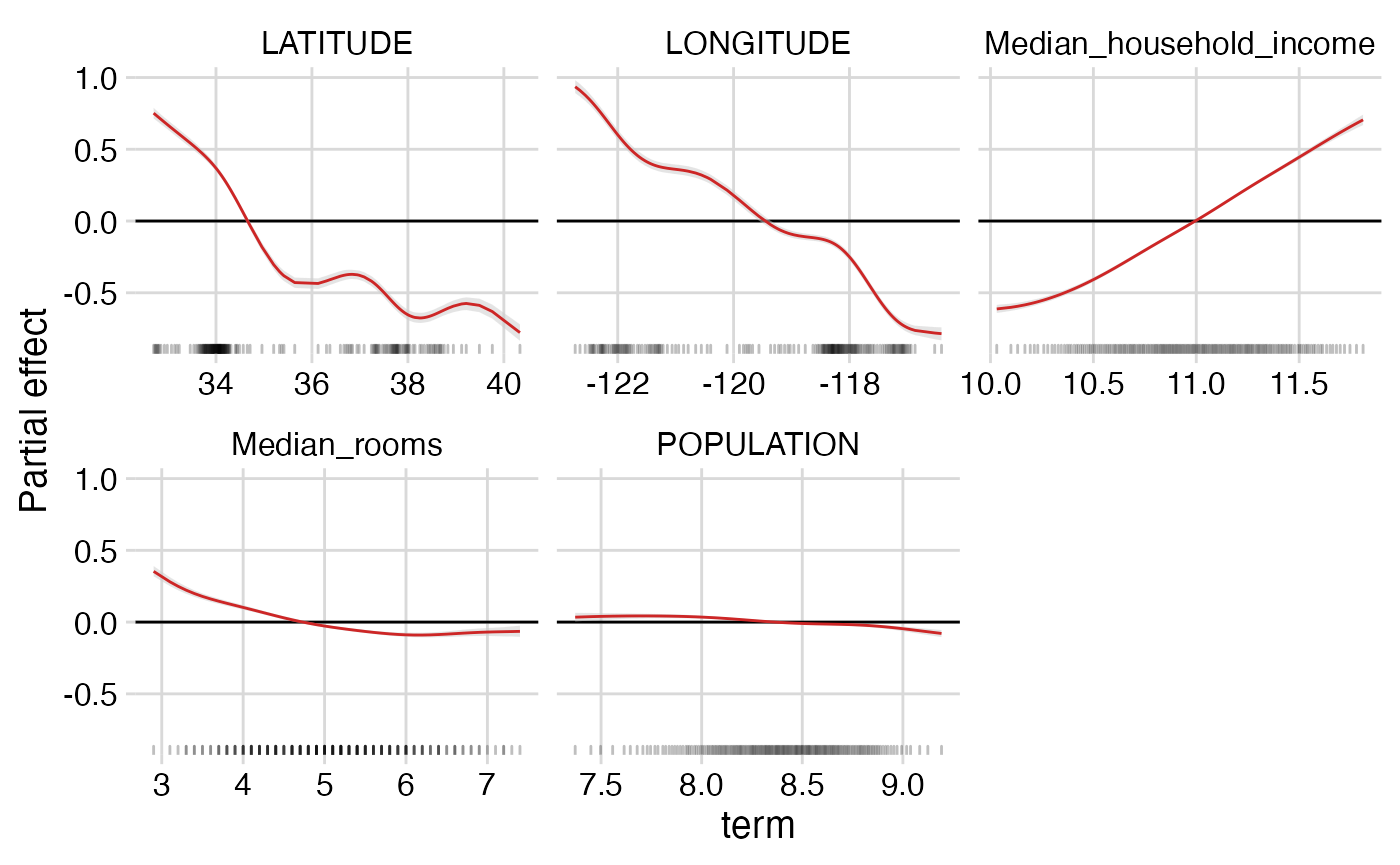
Look at triangles:
additive_summary_triangle_plot(mypossum)
additive_summary_triangle_plot(mypossum, windsor=0.02)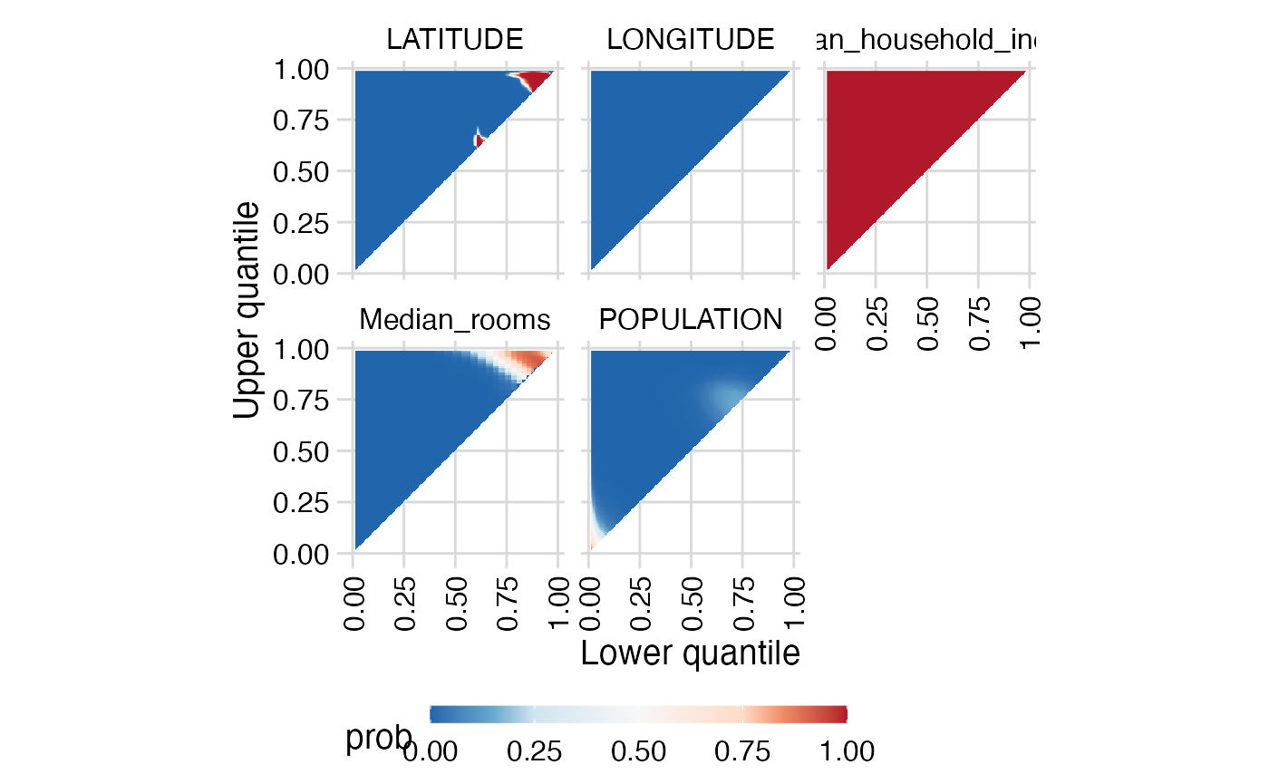
Summary diagnostics
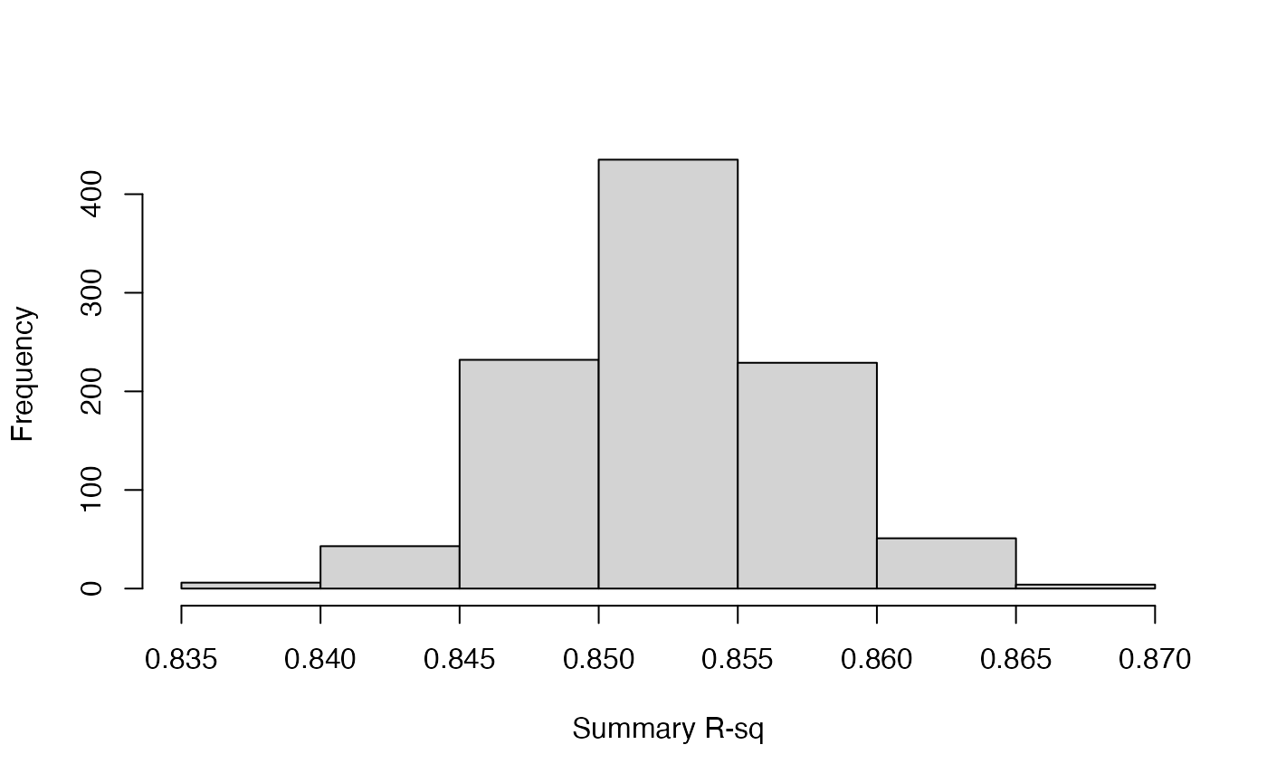
Summary R-sq, i.e., variance explained by summary.
hist(mypossum$summaryRsq, main = "", xlab = "Summary R-sq")