Structure of workflow

1. Get ACS study via tidycensus, which gives sf spatial objects, each with data annotation
2. Get geographic layers via rmapzen
3. Convert geographic layes to sf objects using the sf package
4. Use ggplot2 for vizualization.

Much of this workflow has been taken from a post by Dmitri Shkolnik.

library(sf)
library(ggplot2)
library(cowplot)
theme_set(theme_half_open())

library(tidycensus)
library(sf)
library(dplyr)
library(tigris)
library(rmapzen)

## You need API keys (Census & mapzen) to use these packages.  Don't
## use mine though.

## Get Census API here
## http://api.census.gov/data/key_signup.html

## Get mapzen API here
## https://developers.nextzen.org/

## census_api_key("3deb7c3e77d1747cf53071c077e276d05aa31407", install = TRUE, overwrite = TRUE)
mz_set_tile_host_nextzen(key = ("hxNDKuWbRgetjkLAf_7MUQ"))

## Function for getting map tiles. This, and a lot of other stuff is from:
## https://www.dshkol.com/2018/better-maps-with-vector-tiles/
get_vector_tiles <- function(bbox){
  mz_box=mz_rect(bbox$xmin,bbox$ymin,bbox$xmax,bbox$ymax)
  mz_vector_tiles(mz_box)
}

###############################################################################
                                        #     Get ACS data for geometries     #
###############################################################################

## Income (ACS column B19013_001) & geometry for whole state
# txstateincome <- get_acs(state = "TX", geography = "state", geometry = TRUE,
#                          variables = "B19013_001")

txstateincome <- invisible(get_acs(state = "TX", geography = "state", geometry = TRUE,
                         variables = "B19013_001"))

## Income for state by county
txcountyincome <- invisible(get_acs(state = "TX", geography = "county", geometry = TRUE,
                          variables = "B19013_001") %>%
  arrange(desc(estimate)))

## You can see that we have the shape file (column "geometry") and
## income (column "estimate") for each county
txcountyincome %>% glimpse()

## Plot the counties
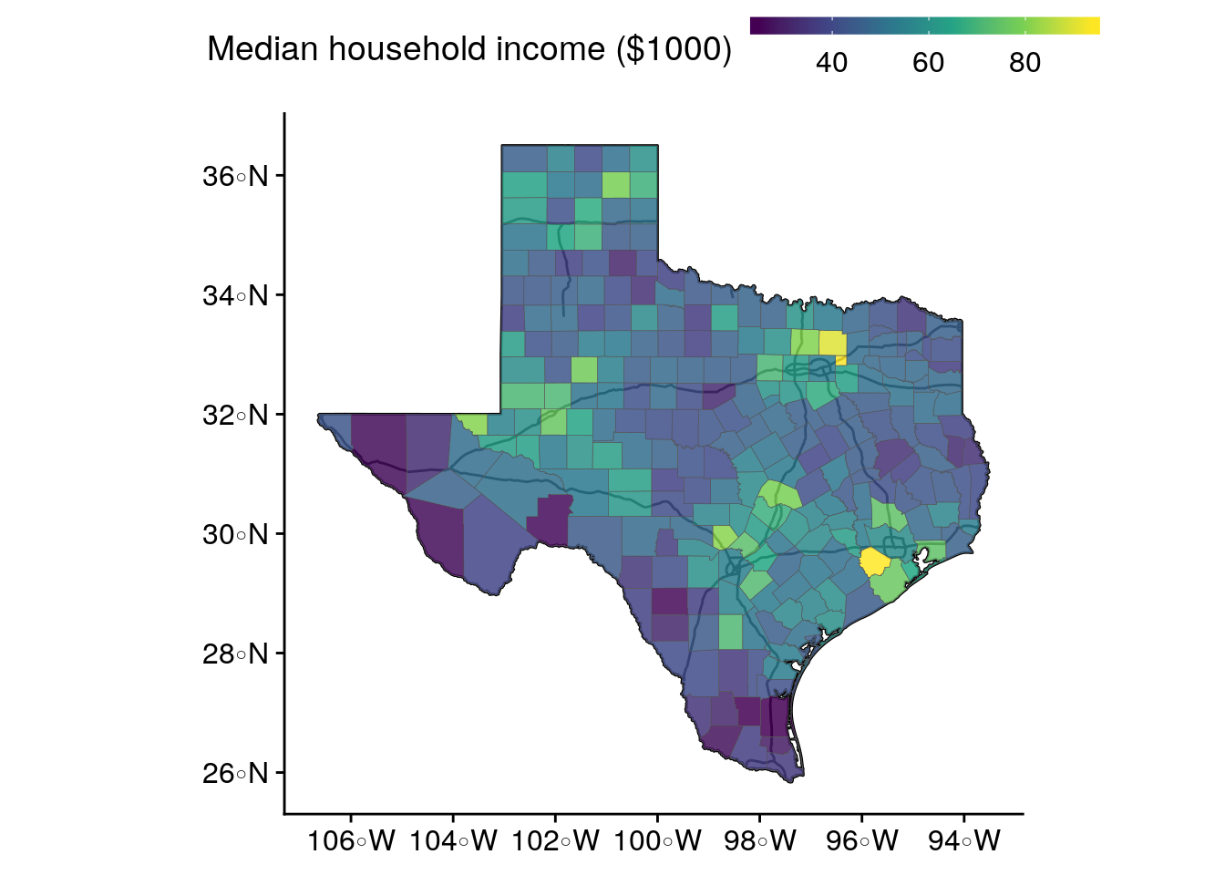
incomeMap <- ggplot(txcountyincome) +
  geom_sf(data = txstateincome, fill = "white", col  = "black") + 
  geom_sf(aes(fill = estimate / 1000), size = 0.1, alpha = 0.8) +
  scale_fill_viridis_c("Median household income ($1000)") +
  theme(legend.position = "top") +
  guides(fill = guide_colorbar(barwidth = 10, barheight = 0.5))

incomeMap

###############################################################################
                                        #  Get geographic info (road & water) #
############################################################################### 

## (this stuff not technically needed, but nice to have as an annotation)

txbbox <- st_bbox(txstateincome)

tx_vector_tiles <- get_vector_tiles(txbbox)
names(tx_vector_tiles)

tx_water <- as_sf(tx_vector_tiles$water)
tx_roads <- as_sf(tx_vector_tiles$roads)

tx_roads_alt <- st_transform(tx_roads, 4269)

txunion <- st_union(txcountyincome$geometry)

tx_roads_crop <- st_intersection(tx_roads_alt, txstateincome)

###############################################################################
                                        # Income plot with roads in background #
###############################################################################

incomeMapRoads <- ggplot() +
  geom_sf(data = txstateincome, fill = "white", col  = "black") +
  geom_sf(data = tx_roads_crop,
          col = "black") +
  geom_sf(data = txcountyincome, aes(fill = estimate / 1000), size = 0.1, alpha = 0.85) +
  theme(legend.position = "top") +
  scale_fill_viridis_c("Median household income ($1000)") +
  guides(fill = guide_colorbar(barwidth = 10, barheight = 0.5))

incomeMapRoads